5 Steps to Crushing Big O
Understanding why Big O notation is important and how to calculate it
Big O notation is a core concept in Computer Science and a frequent, if not obligatory, part of the technical interview process. In a nutshell, Big O notation allows us to figure out the efficiency of algorithms. More specifically, it allows us to measure the time complexity of an algorithm in algebraic terms as its input grows increasingly towards infinity. But why is this important?
Why we use Big O
Imagine asking ten developers to come up with a function that performs a certain task. They all create functions that work perfectly, but how many do you imagine are identical in code? Probably none, especially if the task is moderately complex. So how do you know which function will be the most efficient? Could it be the developer that wrote their function in three lines of code? But what if they have computer from 2006 and have spotty wifi? Will their function run faster than the 20 lines of code on a 2020 laptop?
All the factors above are valid in runtime analysis and almost impossible to answer given the variety of conditions. This is precisely why Big O notation is so important. It strips down the physical factors like speed of the computer’s processor, internet connection, other programs currently executing, etc., and looks at how the algorithm performs as its input increases.
Additionally, because Big O gives us the upper bounds on an algorithm’s running time, what it’s really providing is a worst case scenario. It is answering, “If my function has to go through everything in my input, how long would it take?” Worst case scenario is important here because it is most likely the expected case. Hardly anyone plans for the best case scenario in life, usually just the most likely and the worst. It would be like planning your finances around the possibility of winning the lottery versus the possibility of losing your job.
The same goes for programming. You can certainly plan for the best case scenario when everything is working properly on your site, but what would be most valuable is figuring out how far you can push your code when sh*t hits the fan. This happens everyday and we need not look farther than any site currently trying to sell the new PS5 game console. Those that crash or run incredibly slow are experiencing their worst case scenario, both in terms of Big O and their bottom line. After all, a customer will only use your services as long as they work and work efficiently.
General concepts
When it comes to figuring out the Big O of an algorithm, it takes some practice but can be easily mastered with the following five steps.
Step #1: Count the steps
Let’s take a look at the code below. Would there be a runtime difference if items_array contained 5 elements vs 10000000 elements?

If you said “No”, you are correct! The reason is because no matter how the input grows, this function is only ever doing one thing — printing out the first element in the array. This is what we would call O(1) which represents “constant time”. Similarly, if you have a function that does nothing with the input, such as the code below, it would also have constant time.

Now, say we had a function that went through a loop. This means that no matter what, we are guaranteed to go through each item of the loop at least once, depending on what the function is trying to achieve. If we have a single loop, like in the code below, we would call this O(n), or “linear time”, because the runtime will increase linearly as the input increases. This means that if we have 5 elements in an array, we would print all 5 elements. If the array input was 1000, then we would print it 1000 times.

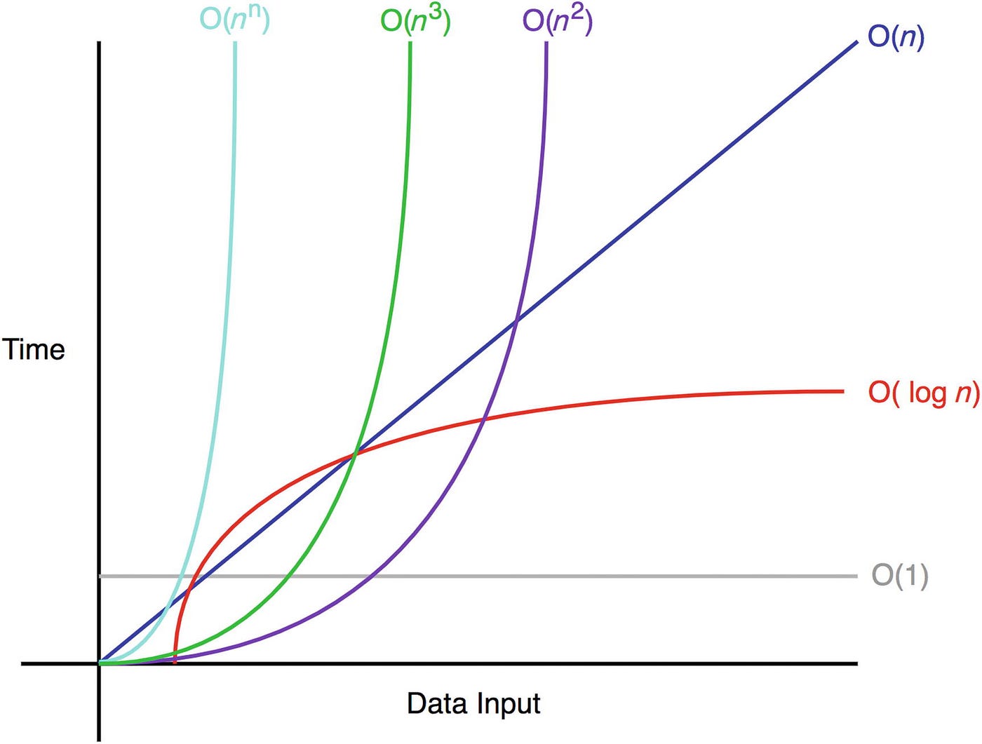
This linear runtime is represented in the chart below in green. See how the time increases at a steady and predictable rate as the data input grows? That is what linear means, a straight line! If we think back to our previous O(1), or constant time, example, we see that the runtime stays, well, constant no matter how much our data input, n, grows.

So when we think of steps, think of it in terms of what we are doing with the input and how that would change with size. We’ve covered what O(1) and O(n) would look like, but there are numerous other types of Big O runtimes.
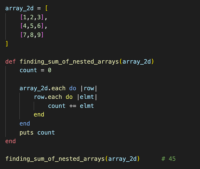
Quadratic time, or O(n²), for example, is commonly found if you are making your way through 2 nested loops. If we look at the example below, we can see that the function finding_sum_of_nested_arrays is taking a two-dimensional array (an array of arrays), array_2d, and looping through each row and then each element to get the sum. Here, we can describe the outer loop as running n times and the inner loop as running n times for every outer loop iteration, or n².
If you see a function with 3 nested loops, then it will likely be O(n³) or cubic time. Four nested loops would be O(n⁴) and so on.
When in doubt just add the number of nested loops and you should be on a good path.
Step #2: Different steps get added
Ok, so we’ve had a quick introduction into loops, but what about algorithms that have more than one thing going on? Great question! One important thing to remember about Big O is that n has to mean something. If you are dealing with more than one something, then you are going to need more than one variable. Also, n is just a common practice variable but we can easily describe all of the functions we’ve seen so far as something else, like O(4), O(a), O(b²), etc.
So let’s take a look at the following function.
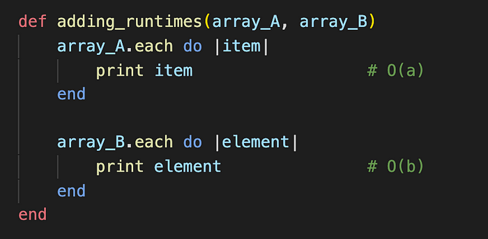
Similar to our previous examples, we are dealing with two loops in one function. This function, however, does not have the loops nested. Instead, we loop through array_A, print the results, then move on to array_B and do the same thing. In this example, we need two variables to describe what is going on because we are taking the runtime for each input. Here, the two inputs are independent of each other and do not compound, so our time complexity would be O(a + b).
The temptation to multiply the two inputs, or O(a*b), is strong, but we must remember that Big O is about how the algorithm scales as the inputs increase. In the scenario above, array_A is not effected if array_B grows, so we must treat them as two distinct variables. Gayle Laakmann McDowell, author of “Cracking the Coding Interview”, put it best:
“If your algorithm is in the form ‘do this, then, when you’re all done, do that’ then you add the runtimes. If your algorithm is in the form ‘do this for each time you do that’ then you multiply the runtimes.”
Step#3: Drop constants and coefficients
Yup, you read that right! When it comes to Big O, we don’t care about constants or coefficients because what we are really after is how the function scales.
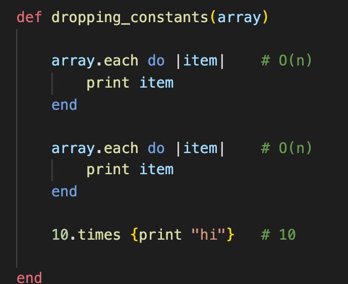
Take, for example, the code above which can be described as O( 2n +10), with 2n coming from two loops executing the single array and 10 from the last line that prints out hi ten times. Even though we might be tempted to say definitively that it is O( 2n +10) and nothing else, we would be incorrect. Again, we care about the scale of this algorithm so we need to drop the constants and the coefficients first.
What is a constant? In this case, it is 10 in O( 2n +10). This makes sense to drop because 10 will never change even if our input of array increases by 1000%.
So now we are left with O(2n). In this case, 2 is our coefficient meaning that it is a numerical value which we are multiplying our variable by. Again, we are interested in the scale of our algorithm so saying O(2n) vs O(10n) vs O(n) does not change the fact that it will always have a linear runtime.
At the end of the day, neither constants nor coefficients play a significant role as our data input, n, gets closer to infinity.
Step#4: Drop non-dominant terms
Ok, so this one seems a little tricky and counter intuitive but stay with me. Let’s say we have an algorithm we’ve calculated as O(n² + 4n³), how can we pare this down?
First, we want to go for the low-hanging fruit and get rid of the coefficient 4 for reasons previously discussed. Now we are left with O(n² + n³). Remember that Big O is all about scale, so we want to drop the non-dominant term, aka the part(s) of the expression that play a less significant role as our input increases. In this case, our non-dominant term would be n², leaving us with O(n³) as our runtime. Let’s put this in terms of numbers:
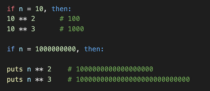
In the first example, we set n = 10. When we square n (n² or n ** 2), the result is 100. If we cube n (n³ or n ** 3), our result is 1000, just 10x more than n². That doesn’t seem like a lot but see what happens in our second example when n = 1,000,000,000. Now the difference between n² and n³ is much more significant and we can see that n³ will only continue to eclipse n² more and more as we approach infinity.
Step #5: Different inputs get different variables
Finally, when dealing with multiple inputs, we must remember to use multiple variables. After all, n in O(n) is a data input, not just a random letter someone decided to stick between parenthesis. If we have multiple data inputs then they each must have their own unique variable to acknowledge their relationship.
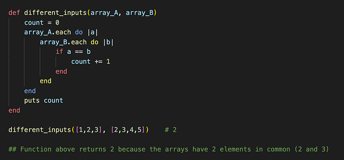
In the function above, we have two arrays, array_A and array_B. Here we are saying “for every element in array_A, go through all of the elements in array_B. Therefore, this function’s runtime can be described as O(a*b) because the length of each loop is multiplied by the length of the other.
Conclusion
Big O can be tricky and, frankly, I am still on my way to really understanding this concept. There are a host of resources and tutorials out there in the world and I highly recommend you comb through them to get a better grasp of what is going on with Big O. I didn’t even touch on a handful of common runtimes, such as O(x!), O(x log x), or O(log x), but I highly recommend reading more about them as they will likely pop up in any leetcode data structure questions or even technical interviews. If I figure out what they mean, perhaps there will be a sequel to this post…
As always, thanks for reading! If you have any comments or suggestions on how to make this article better, please feel free to comment. Thanks!
Resources
Below are some of the resources I found helpful in tackling the basics of Big O notation.
- “Cracking the Coding Interview” by Gayle Laakmann McDowell
- Interview Cake, Big O Notation and Time Complexity
- Khan Academy, Big O notation
- Khan Academy, Functions in asymptotic notation
